We solve
![]()
![]()
>function f([x,y]) &= [x^2+y^2-10,x+y-1]
                        2    2
                      [y  + x  - 10, y + x - 1]
Euler can plot the solutions of both equations.
>plot2d(&f(x,y)[1],level=0,r=5); ...
 plot2d(&f(x,y)[2],level=0,add=true):
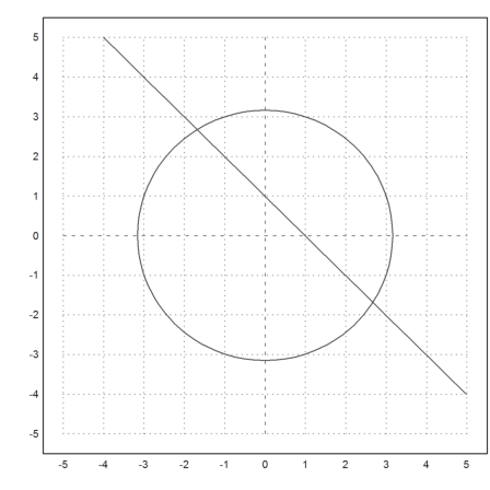
The intersections are the solutions.
To start the Newton algorithm we need the Jacobian.
>function Df([x,y]) &= jacobian(f(x,y),[x,y])
                             [ 2 x  2 y ]
                             [          ]
                             [  1    1  ]
Now, there is the newton2 function, which does the iteration.
It needs to function f(v) and Df(v). That is, why we define f and Df with f([x,y]) and Df([x,y]). Those functions can be used with vectors or two elements.
>newton2("f","Df",[-3,3])
[-1.67945, 2.67945]
We want to simulate the Newton iteration step by step. So we define the iterating function.
>function fiter ([x,y]) &= [x,y]-invert(Df(x,y)).f(x,y)
               [    2    2                            ]
               [ - y  - x  + 10   2 y (y + x - 1)     ]
               [ -------------- + --------------- + x ]
               [   2 x - 2 y         2 x - 2 y        ]
               [                                      ]
               [   2    2                             ]
               [  y  + x  - 10   2 x (y + x - 1)      ]
               [  ------------ - --------------- + y  ]
               [   2 x - 2 y        2 x - 2 y         ]
>&factor(fiter(x,y))
                       [    2          2      ]
                       [ - y  + 2 y - x  - 10 ]
                       [ -------------------- ]
                       [      2 (y - x)       ]
                       [                      ]
                       [   2    2             ]
                       [  y  + x  - 2 x + 10  ]
                       [  ------------------  ]
                       [      2 (y - x)       ]
Maxima returns a column vector. We need a row vector as input and output. So we define an iteration function g.
>function g(v) := fiter(v)'
Then we can iterate using the iterate() function.
>iterate("g",[-3.2,3],10)
         -3.2             3
     -1.87419       2.87419
     -1.68744       2.68744
     -1.67946       2.67946
     -1.67945       2.67945
     -1.67945       2.67945
     -1.67945       2.67945
     -1.67945       2.67945
     -1.67945       2.67945
     -1.67945       2.67945
     -1.67945       2.67945
Another starting point yields the other solution.
>iterate("g",[1,-2],10)
            1            -2
      3.16667      -2.16667
      2.72396      -1.72396
      2.67989      -1.67989
      2.67945      -1.67945
      2.67945      -1.67945
      2.67945      -1.67945
      2.67945      -1.67945
      2.67945      -1.67945
      2.67945      -1.67945
      2.67945      -1.67945
Of course, we can also solve this example symbolically.
>&solve(f(x,y)), %()
             1 - sqrt(19)      sqrt(19) + 1
       [[y = ------------, x = ------------],
                  2                 2
                                      sqrt(19) + 1      1 - sqrt(19)
                                 [y = ------------, x = ------------]]
                                           2                 2

[-1.67945,  2.67945,  2.67945,  -1.67945]
There is also the Broyden algorithm, which does not need the derivative. It is a generalization of the Secant algorithm for more then one variable.
>broyden("f",[-3,2])
[-1.67945, 2.67945]
With the interval Newton method, we even get a proved inclusion of the zero.
>inewton2("f","Df",[-3,1])
[ ~-1.679449471770339,-1.679449471770335~,
~2.679449471770335,2.679449471770338~ ]